Evaluate a golden codec on your own data

Download notebookView sourceOpen in Colab

Open in Colab opens the source notebook only. Before running cells, use a Python 3.12 runtime and install compressionKIT into that runtime. See notebook environment setup. Hosted execution has not been validated by this documentation build.

This example displays saved outputs. Building the documentation does not run training. Check dataset paths for your notebook working directory before running.

Score a published compressionKIT codec on signals you provide — either your own recordings or the built-in synthetic generators (no dataset needed).

The flow is the same regardless of source:

1. Load a codec.
2. Get a 1-D signal sampled at codec.sample_rate Hz.
3. Split into codec.frame_size frames, round-trip, and aggregate metrics.

Python

import matplotlib.pyplot as plt
import numpy as np
import pandas as pd

from compressionkit.evaluation.metrics import compute_signal_metrics
from compressionkit.runtime import load_codec
from compressionkit.synthetic import add_noise, ecg_mcsharry, ppg_dynamical

# "-v1.0" repos are the current release track. Uncomment any line below to
# try a different modality/compression ratio or codec family (RVQ = learned/AI,
# SPIHT = DSP-only wavelet codec, hybrid = learned denoiser + SPIHT). All three
# families implement the same Codec interface, so nothing below needs to change.
CODEC_SOURCE = "Ambiq/compressionkit-ppg-4x-v1.0"
# CODEC_SOURCE = "Ambiq/compressionkit-ppg-2x-v1.0"
# CODEC_SOURCE = "Ambiq/compressionkit-ppg-8x-v1.0"
# CODEC_SOURCE = "Ambiq/compressionkit-ppg-16x-v1.0"
# CODEC_SOURCE = "Ambiq/compressionkit-ppg-32x-v1.0"
# CODEC_SOURCE = "Ambiq/compressionkit-ecg-2x-v1.0"
# CODEC_SOURCE = "Ambiq/compressionkit-ecg-4x-v1.0"
# CODEC_SOURCE = "Ambiq/compressionkit-ecg-8x-v1.0"
# CODEC_SOURCE = "Ambiq/compressionkit-ecg-16x-v1.0"
# CODEC_SOURCE = "Ambiq/compressionkit-ecg-32x-v1.0"
# CODEC_SOURCE = "Ambiq/compressionkit-ecg-64x-v1.0"
# SPIHT (DSP-only, no trained weights) and hybrid (learned denoiser + SPIHT):
# CODEC_SOURCE = "Ambiq/compressionkit-ppg-spiht-4x-v1.0"
# CODEC_SOURCE = "Ambiq/compressionkit-ppg-hybrid-4x-v1.0"
# CODEC_SOURCE = "Ambiq/compressionkit-ecg-spiht-4x-v1.0"
# CODEC_SOURCE = "Ambiq/compressionkit-ecg-hybrid-4x-v1.0"
# CODEC_SOURCE = "results/ppg_rvq_64hz_04x_golden/deploy"  # local, offline

codec = load_codec(CODEC_SOURCE)
fs, n = codec.sample_rate, codec.frame_size
print(f"{codec.name}  ({codec.modality}, {fs} Hz, {n}-sample frames)")

Saved output

Fetching 15 files: 100%|██████████| 15/15 [00:00<00:00, 14328.07it/s]

Saved output

ppg_rvq_64hz_04x_golden  (ppg, 64 Hz, 320-sample frames)

Option A — synthetic signal (runs anywhere)

The analytical generators produce a clean, ground-truth waveform at the codec’s sample rate. Add calibrated noise to mimic real wearables.

Python

duration_s = 60.0
if codec.modality == "ecg":
    clean = ecg_mcsharry(duration_s=duration_s, sample_rate=float(fs), hr_mean=60.0)
else:
    clean = ppg_dynamical(duration_s=duration_s, sample_rate=float(fs), hr_mean=72.0)

# Optional: add noise at a single target SNR to stress-test the codec.
# For a sweep across several noise levels at once, see the "Robustness"
# section below instead.
# clean, _ = add_noise(clean, sample_rate=float(fs), snr_db=15.0)

signal = clean.astype("float32")
print(f"signal: {signal.shape[0]} samples ({signal.shape[0] / fs:.1f} s)")

Saved output

signal: 3840 samples (60.0 s)

Option B — bring your own data

Provide a 1-D float32 array sampled at codec.sample_rate Hz (resample first if your sensor runs at a different rate). Uncomment to use it instead of the synthetic signal above.

Python

# signal = np.load("my_recording.npy").astype("float32")
# assert signal.ndim == 1, "expects a 1-D signal at codec.sample_rate Hz"
#
# If your data is at a different rate, resample to codec.sample_rate first:
# from scipy.signal import resample_poly
# signal = resample_poly(signal, fs, native_fs).astype("float32")

Frame, round-trip, and score

Python

def to_frames(sig: np.ndarray, frame_size: int) -> np.ndarray:
    """Split a 1-D signal into non-overlapping (n_frames, frame_size) frames."""
    usable = (len(sig) // frame_size) * frame_size
    return sig[:usable].reshape(-1, frame_size)


frames = to_frames(signal, n)
rows, recon_frames = [], []
for i, f in enumerate(frames):
    enc = codec.compress(f)
    rec = codec.decompress(enc)
    recon_frames.append(rec)
    mm = compute_signal_metrics(f, rec)
    rows.append({
        "frame": i,
        "bits": enc.nbits,
        "prd_percent": mm["prd_percent"],
        "cosine_similarity": mm["cosine_similarity"],
        "rmse": mm["rmse"],
    })

df = pd.DataFrame(rows)
recon = np.concatenate(recon_frames)
overall_cr = (frames.size * 32) / df["bits"].sum()  # vs 32-bit float baseline

print(f"frames     : {len(df)}")
print(f"overall CR : {overall_cr:.2f}x (vs 32-bit float)")
df[["prd_percent", "cosine_similarity", "rmse"]].describe().loc[["mean", "50%", "min", "max"]]

Saved output

frames     : 12
overall CR : 4.00x (vs 32-bit float)

Saved output

      prd_percent  cosine_similarity      rmse
mean    16.585491           0.987021  0.009096
50%     16.809828           0.986869  0.009187
min     12.790186           0.983588  0.008409
max     18.440839           0.991917  0.009915

Python

fig, ax = plt.subplots(2, 1, figsize=(10, 5))

show = slice(0, min(5 * n, len(signal)))  # first ~5 frames
t = np.arange(len(recon))[show] / fs
ax[0].plot(t, signal[: len(recon)][show], label="original", lw=1.4)
ax[0].plot(t, recon[show], label="reconstruction", lw=1.1, alpha=0.85)
ax[0].set_title(f"{codec.name}  ·  median PRD {df['prd_percent'].median():.2f}%  ·  CR {overall_cr:.2f}x")
ax[0].set_xlabel("time (s)")
ax[0].legend()

ax[1].hist(df["prd_percent"], bins=30, color="#4C78A8")
ax[1].axvline(df["prd_percent"].median(), color="k", ls="--")
ax[1].set_xlabel("PRD %")
ax[1].set_ylabel("frames")
ax[1].set_title("Per-frame PRD distribution")

plt.tight_layout()
plt.show()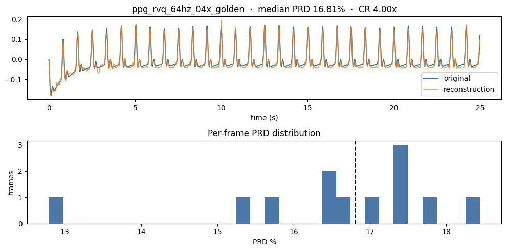

Saved output · cell 9

Robustness: fidelity across noise levels

A single pass hides how the codec degrades as input quality drops. Sweep a small SNR ladder using the same calibrated noise harness the golden models are evaluated with, and edit snr_levels_db to add more/finer levels.

If you have real recorded noise segments (not synthetic), use compressionkit.evaluation.empirical_regime.add_empirical_noise(windows, noise_bank, snr_db, seed=...) instead — this is the literal empirical-noise injection used by golden training/eval, but it requires your own noise_bank array of real noise/residual segments.

Python

snr_levels_db: list[float | None] = [None, 24, 18, 12, 6, 0]  # None = clean; add/remove levels freely

snr_rows = []
for snr_db in snr_levels_db:
    if snr_db is None:
        noisy_signal, label = signal, "clean"
    else:
        noisy_signal, _ = add_noise(signal, sample_rate=float(fs), snr_db=snr_db, seed=0)
        noisy_signal = noisy_signal.astype("float32")
        label = f"{snr_db:g} dB"

    noisy_frames = to_frames(noisy_signal, n)
    prd_vals = [compute_signal_metrics(f, codec.decompress(codec.compress(f)))["prd_percent"] for f in noisy_frames]
    snr_rows.append({"input": label, "median_prd_percent": float(np.median(prd_vals)), "frames": len(prd_vals)})

snr_df = pd.DataFrame(snr_rows)
snr_df

Saved output

   input  median_prd_percent  frames
0  clean           16.809828      12
1  24 dB           17.206760      12
2  18 dB           18.011693      12
3  12 dB           22.661638      12
4   6 dB           33.776077      12
5   0 dB           49.759792      12

Python

plt.figure(figsize=(8, 4))
plt.plot(range(len(snr_df)), snr_df["median_prd_percent"], marker="o")
plt.xticks(range(len(snr_df)), snr_df["input"])
plt.xlabel("input condition")
plt.ylabel("median PRD %")
plt.title(f"{codec.name}: fidelity vs. input noise level")
plt.grid(alpha=0.3)
plt.tight_layout()
plt.show()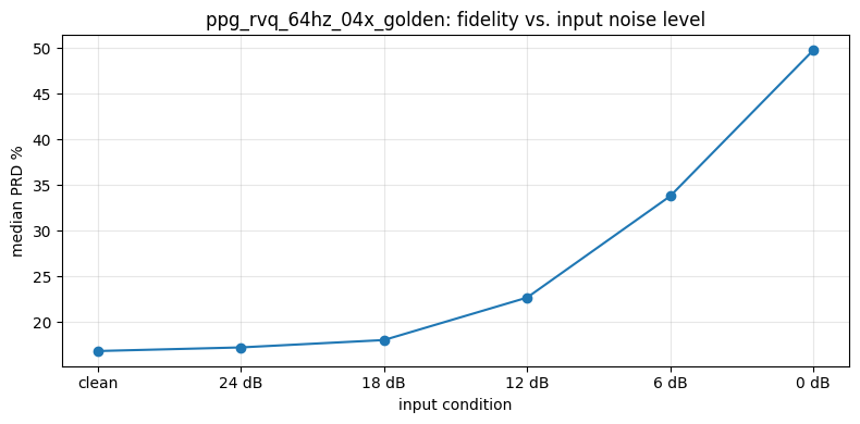

Saved output · cell 12

Next steps

• Compare available tiers on the same signal to pick a CR/fidelity operating point.
• Extend the noise sweep above with more levels, or plug in real recorded noise via add_empirical_noise.
• Set up real datasets via the Dataset Setup guide for population-scale evaluation.