Train ECG Arrhythmia Classifier
This example displays saved outputs. Building the documentation does not run training. Check dataset paths for your notebook working directory before running.
Date created: 2024/07/17
Last Modified: 2024/07/17
Description: Train, evaluate, and export 4-stage ECG arrhythmia classifier
Overview
Section titled “Overview”In this guide, we will train an ECG-based arrhythmia classifier that uses an EfficientNetV2 inspired model. The classifier is trained on raw ECG data and is able to discern normal sinus rhythm (NSR), sinus bradycardia (SBRAD), atrial fibrillation (AFIB), and general supraventricular tachycardia (GSVT).
Input
- Sensor: ECG
- Location: Wrist
- Sampling Rate: 100 Hz
- Frame Size: 5 seconds
Class Mapping
Identify rhythm into one of four categories: SR, SBRAD, AFIB, GSVT.
| Base Class | Target Class | Label |
|---|---|---|
| 0-SR | 0 | Sinus Rhythm (SR) |
| 1-SBRAD | 1 | Sinus Bradycardia (SBRAD) |
| 7-AFIB, 8-AFL | 2 | AFIB/AFL (AFIB) |
| 2-STACH, 5-SVT | 3 | General supraventricular tachycardia (GSVT) |
Datasets
- LSAD: The Large Scale Rhythm Database (LSAD) is a large publicly available electrocardiography dataset. It contains 10 second, 12-lead ECGs of 45,152 patients with a 500 Hz sampling rate. The ECGs are sampled at 500 Hz and are annotated by up to two cardiologists.
import os
os.environ["TF_CPP_MIN_LOG_LEVEL"] = "3"import IPythonimport contextlibfrom pathlib import Pathimport tempfileimport kerasimport heartkit as hkimport helia_edge as helia
# Be sure to set the dataset path to the correct locationdatasets_dir = Path(os.getenv("HK_DATASET_PATH", "./datasets"))
plot_theme = hk.utils.dark_themehelia.utils.silence_tensorflow()hk.utils.setup_plotting(plot_theme)logger = helia.utils.setup_logger(__name__)Configure datasets
Section titled “Configure datasets”We are going to train our model using the Large scale Arrhythmia dataset. This dataset uses the slug lsad within heartKIT. We will download the dataset if it is not already available.
datasets = [ hk.NamedParams( name="lsad", params=dict( path=datasets_dir / "lsad", ), )]Target classes
Section titled “Target classes”For this task, we are going to classify ECG signals into one of four classes:
- Sinus Rhytm: Normal ECG signal (SR)
- Sinus Bradycardia: Slow heart rate (SB)
- Atrial Flutter/Fibrillation: Irregular heart rate (AFIB)
- General Supra-Ventricular Tachycardia: Fast heart rate (GSVT)
heartKIT already provides a number of heart rhythms. We will provide a class mapping for the four classes we are interested in. We will also provide class names for display purposes.
class_map = {    hk.tasks.HKRhythm.sr: 0,    hk.tasks.HKRhythm.sbrad: 1,    hk.tasks.HKRhythm.afib: 2,    hk.tasks.HKRhythm.aflut: 2,    hk.tasks.HKRhythm.stach: 3,    hk.tasks.HKRhythm.svt: 3,}
class_names = ["SR", "SB", "AFIB", "GSVT"]
Preprocess pipeline
Section titled “Preprocess pipeline”We will preprocess the ECG signals by applying the following steps:
- Apply Z-score normalization w/ epsilon to avoid division by zero
The task accepts a list of preprocessing functions that will be applied to the input data.
preprocesses = [hk.NamedParams(name="layer_norm", params=dict(epsilon=0.01, name="znorm"))]Define EfficientNetV2 model architecture
Section titled “Define EfficientNetV2 model architecture”For this task, we are going to leverage a customized EfficientNetV2 model architecture that is smaller and can handle 1D signals. The model consists of 6 MBConv style blocks with a depth of 2. Each block leverages squeeze-and-excitation mechanism w/ ratio of 4 to improve the model’s performance.
architecture = hk.NamedParams( name="efficientnetv2", params=dict( input_filters=24, input_kernel_size=(1, 9), input_strides=(1, 2), blocks=[ dict(filters=24, depth=1, kernel_size=(1, 9), strides=(1, 2), ex_ratio=1, se_ratio=4), dict(filters=32, depth=1, kernel_size=(1, 9), strides=(1, 2), ex_ratio=1, se_ratio=4), dict(filters=48, depth=1, kernel_size=(1, 9), strides=(1, 2), ex_ratio=1, se_ratio=4), dict(filters=64, depth=1, kernel_size=(1, 9), strides=(1, 2), ex_ratio=1, se_ratio=4), dict(filters=80, depth=1, kernel_size=(1, 9), strides=(1, 2), ex_ratio=1, se_ratio=4), dict(filters=96, depth=1, kernel_size=(1, 9), strides=(1, 2), ex_ratio=1, se_ratio=4), ], output_filters=0, include_top=True, use_logits=True, ),)Task configuration
Section titled “Task configuration”Here we provide the complete configuration for the task. This includes the dataset configuration, preprocessing pipeline, model architecture, and training parameters.
params = hk.HKTaskParams( # Common arguments name="hk-4-stage-rhythm", job_dir=Path(tempfile.gettempdir()) / "hk-4-stage-rhythm", # Dataset arguments datasets=datasets, # Signal arguments sampling_rate=100, frame_size=800, # Dataloader arguments samples_per_patient=5, val_samples_per_patient=5, test_samples_per_patient=5, # Preprocessing/Augmentation arguments preprocesses=preprocesses, # Class arguments num_classes=len(class_names), class_map=class_map, class_names=class_names, # Split arguments val_patients=0.2, val_size=20000, test_size=20000, val_file="val.tfds", test_file="val.tfds", # Model arguments model_file="model.keras", architecture=architecture, # Training parameters lr_rate=1e-3, lr_cycles=1, batch_size=256, buffer_size=25000, epochs=100, steps_per_epoch=50, val_metric="loss", class_weights="balanced", # Evaluation arguments threshold=0.5, test_metric_threshold=0.98, # Export parameters tflm_var_name="ecg_rhythm_flatbuffer", tflm_file="ecg_rhythm_flatbuffer.h", # Demo params backend="pc", demo_size=800, display_report=False, # Extra arguments verbose=1, seed=42,)Load rhythm task
Section titled “Load rhythm task”heartKIT provides a TaskFactory that includes a number ready-to-use tasks. Each task provides methods for training, evaluating, exporting, and demoing. We will grab the rhythm task and configure it for our use case.
task = hk.TaskFactory.get("rhythm")Download datasets
Section titled “Download datasets”We will download the datasets needed for the task.
task.download(params=params)Visualize the model
Section titled “Visualize the model”Lets quickly instantiate and visualize the first few layers of the model.
model = helia.models.efficientnet.efficientnetv2_from_object( x=keras.Input(shape=(params.frame_size, 1), name="inputs"), params=architecture.params, num_classes=len(class_names))model.summary(layer_range=("inputs", model.layers[10].name))WARNING: All log messages before absl::InitializeLog() is called are written to STDERRI0000 00:00:1723841711.256117 789182 cuda_executor.cc:1015] successful NUMA node read from SysFS had negative value (-1), but there must be at least one NUMA node, so returning NUMA node zero. See more at https://github.com/torvalds/linux/blob/v6.0/Documentation/ABI/testing/sysfs-bus-pci#L344-L355I0000 00:00:1723841711.276561 789182 cuda_executor.cc:1015] successful NUMA node read from SysFS had negative value (-1), but there must be at least one NUMA node, so returning NUMA node zero. See more at https://github.com/torvalds/linux/blob/v6.0/Documentation/ABI/testing/sysfs-bus-pci#L344-L355I0000 00:00:1723841711.276664 789182 cuda_executor.cc:1015] successful NUMA node read from SysFS had negative value (-1), but there must be at least one NUMA node, so returning NUMA node zero. See more at https://github.com/torvalds/linux/blob/v6.0/Documentation/ABI/testing/sysfs-bus-pci#L344-L355I0000 00:00:1723841711.278058 789182 cuda_executor.cc:1015] successful NUMA node read from SysFS had negative value (-1), but there must be at least one NUMA node, so returning NUMA node zero. See more at https://github.com/torvalds/linux/blob/v6.0/Documentation/ABI/testing/sysfs-bus-pci#L344-L355I0000 00:00:1723841711.278130 789182 cuda_executor.cc:1015] successful NUMA node read from SysFS had negative value (-1), but there must be at least one NUMA node, so returning NUMA node zero. See more at https://github.com/torvalds/linux/blob/v6.0/Documentation/ABI/testing/sysfs-bus-pci#L344-L355I0000 00:00:1723841711.278176 789182 cuda_executor.cc:1015] successful NUMA node read from SysFS had negative value (-1), but there must be at least one NUMA node, so returning NUMA node zero. See more at https://github.com/torvalds/linux/blob/v6.0/Documentation/ABI/testing/sysfs-bus-pci#L344-L355I0000 00:00:1723841711.327697 789182 cuda_executor.cc:1015] successful NUMA node read from SysFS had negative value (-1), but there must be at least one NUMA node, so returning NUMA node zero. See more at https://github.com/torvalds/linux/blob/v6.0/Documentation/ABI/testing/sysfs-bus-pci#L344-L355I0000 00:00:1723841711.327778 789182 cuda_executor.cc:1015] successful NUMA node read from SysFS had negative value (-1), but there must be at least one NUMA node, so returning NUMA node zero. See more at https://github.com/torvalds/linux/blob/v6.0/Documentation/ABI/testing/sysfs-bus-pci#L344-L355I0000 00:00:1723841711.327833 789182 cuda_executor.cc:1015] successful NUMA node read from SysFS had negative value (-1), but there must be at least one NUMA node, so returning NUMA node zero. See more at https://github.com/torvalds/linux/blob/v6.0/Documentation/ABI/testing/sysfs-bus-pci#L344-L355Model: "EfficientNetV2"Saved output
┏━━━━━━━━━━━━━━━━━━━━━┳━━━━━━━━━━━━━━━━━━━┳━━━━━━━━━━━━┳━━━━━━━━━━━━━━━━━━━┓┃ Layer (type) ┃ Output Shape ┃ Param # ┃ Connected to ┃┡━━━━━━━━━━━━━━━━━━━━━╇━━━━━━━━━━━━━━━━━━━╇━━━━━━━━━━━━╇━━━━━━━━━━━━━━━━━━━┩│ inputs (InputLayer) │ (None, 800, 1) │ 0 │ - │├─────────────────────┼───────────────────┼────────────┼───────────────────┤│ reshape (Reshape) │ (None, 1, 800, 1) │ 0 │ inputs[0][0] │├─────────────────────┼───────────────────┼────────────┼───────────────────┤│ stem.conv (Conv2D) │ (None, 1, 400, │ 216 │ reshape[0][0] ││ │ 24) │ │ │├─────────────────────┼───────────────────┼────────────┼───────────────────┤│ stem.bn │ (None, 1, 400, │ 96 │ stem.conv[0][0] ││ (BatchNormalizatio… │ 24) │ │ │├─────────────────────┼───────────────────┼────────────┼───────────────────┤│ stem.act │ (None, 1, 400, │ 0 │ stem.bn[0][0] ││ (Activation) │ 24) │ │ │├─────────────────────┼───────────────────┼────────────┼───────────────────┤│ stage1.mbconv1.dp │ (None, 1, 400, │ 216 │ stem.act[0][0] ││ (DepthwiseConv2D) │ 24) │ │ │├─────────────────────┼───────────────────┼────────────┼───────────────────┤│ stage1.mbconv1.dp.… │ (None, 1, 400, │ 96 │ stage1.mbconv1.d… ││ (BatchNormalizatio… │ 24) │ │ │├─────────────────────┼───────────────────┼────────────┼───────────────────┤│ stage1.mbconv1.dp.… │ (None, 1, 400, │ 0 │ stage1.mbconv1.d… ││ (Activation) │ 24) │ │ │├─────────────────────┼───────────────────┼────────────┼───────────────────┤│ max_pooling2d │ (None, 1, 200, │ 0 │ stage1.mbconv1.d… ││ (MaxPooling2D) │ 24) │ │ │├─────────────────────┼───────────────────┼────────────┼───────────────────┤│ stage1.mbconv1.se.… │ (None, 1, 1, 24) │ 0 │ max_pooling2d[0]… ││ (GlobalAveragePool… │ │ │ │├─────────────────────┼───────────────────┼────────────┼───────────────────┤│ stage1.mbconv1.se.… │ (None, 1, 1, 6) │ 150 │ stage1.mbconv1.s… ││ (Conv2D) │ │ │ │└─────────────────────┴───────────────────┴────────────┴───────────────────┘ Total params: 32,192 (125.75 KB) Trainable params: 30,912 (120.75 KB) Non-trainable params: 1,280 (5.00 KB)Train the model
Section titled “Train the model”Now let’s train the model using the LSAD dataset. We will train the model for 100 epochs.
task.train(params)Sorting lsad labels: 100%|██████████| 36120/36120 [00:07<00:00, 4746.99it/s]Sorting lsad labels: 100%|██████████| 36120/36120 [00:07<00:00, 4552.33it/s]INFO Validation steps per epoch: 78 datasets.py:105INFO Saving validation dataset to /tmp/hk-4-stage-rhythm/val.tfds train.py:57Training: 0%| 0/100 ETA: ?s, ?epochs/sWARNING: All log messages before absl::InitializeLog() is called are written to STDERRI0000 00:00:1723841770.965635 789335 service.cc:146] XLA service 0x79d8f400b520 initialized for platform CUDA (this does not guarantee that XLA will be used). Devices:I0000 00:00:1723841770.965656 789335 service.cc:154] StreamExecutor device (0): NVIDIA GeForce RTX 4090, Compute Capability 8.9I0000 00:00:1723841777.014004 789335 device_compiler.h:188] Compiled cluster using XLA! This line is logged at most once for the lifetime of the process.Training: 100%|██████████ 100/100 ETA: 00:00s, 1.94s/epochs78/78 ━━━━━━━━━━━━━━━━━━━━ 1s 806us/step78/78 ━━━━━━━━━━━━━━━━━━━━ 0s 915us/step - acc: 0.9442 - f1: 0.9444 - loss: 0.0903INFO [VAL SET] ACC=0.9444, F1=0.9445, LOSS=0.0920 train.py:190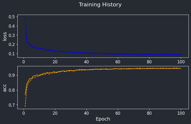
Model evaluation
Section titled “Model evaluation”Now that we have trained the model, we will evaluate the model on the test dataset. Similar to training, we will provide the same task parameters.
task.evaluate(params)INFO Loading validation dataset from /tmp/hk-4-stage-rhythm/val.tfds evaluate.py:3378/78 ━━━━━━━━━━━━━━━━━━━━ 1s 2ms/step - acc: 0.9442 - f1: 0.9444 - loss: 0.0903INFO [TEST SET] ACC=0.9444, F1=0.9445, LOSS=0.0920 evaluate.py:50624/624 ━━━━━━━━━━━━━━━━━━━━ 2s 2ms/step613/613 ━━━━━━━━━━━━━━━━━━━━ 2s 1ms/step - acc: 0.9518 - f1: 0.9520 - loss: 0.0804INFO [TEST SET] THRESH=50.00%, DROP=1.76% evaluate.py:62INFO [TEST SET] ACC=0.9520, F1=0.9521, LOSS=0.0822 evaluate.py:63Confusion matrix
Section titled “Confusion matrix”Let’s visualize the confusion matrix to understand the model’s performance on each class.
IPython.display.Image(filename=params.job_dir / "confusion_matrix_test.png", width=500)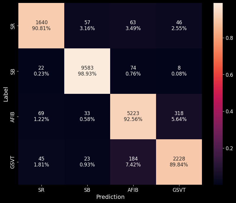
Export model to TF Lite / TFLM
Section titled “Export model to TF Lite / TFLM”Once we have trained and evaluated the model, we need to export the model into a format that can be used for inference on the edge. Currently, we export the model to TensorFlow Lite flatbuffer format. This will also generate a C header file that can be used with TensorFlow Lite for Microcontrollers (TFLM).
Apply post-training quantization (PTQ)
Section titled “Apply post-training quantization (PTQ)”For running on bare metal, we will perform post-training quantization to convert the model to an 8-bit integer model. The weights and activations will be quantized to 8-bits and biases will be quantized to 32-bits. This will reduce the model size and improve the inference speed.
quantization = hk.QuantizationParams( enabled=True, format="INT8", io_type="int8", conversion="KERAS",)params.quantization = quantization# TF dumps a lot of info to stdout, so we redirect it to /dev/nullwith open(os.devnull, "w") as devnull: with contextlib.redirect_stdout(devnull), contextlib.redirect_stderr(devnull): task.export(params=params)W0000 00:00:1723841958.715237 789182 tf_tfl_flatbuffer_helpers.cc:392] Ignored output_format.W0000 00:00:1723841958.715249 789182 tf_tfl_flatbuffer_helpers.cc:395] Ignored drop_control_dependency.INFO Validating model results export.py:94fully_quantize: 0, inference_type: 6, input_inference_type: INT8, output_inference_type: INT8INFO: Created TensorFlow Lite XNNPACK delegate for CPU.INFO [TF METRICS] LOSS=0.2360 ACC=0.9657 F1=0.9761 export.py:101INFO [TFL METRICS] LOSS=0.2441 ACC=0.9639 F1=0.9752 export.py:102INFO Validation passed (0.0080) export.py:110Run inference demo
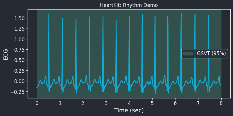
Section titled “Run inference demo”We will run a demo on the PC to verify that the model is working as expected. The demo will load the model and run inferences across a randomly selected ECG signal. The demo will also provide the model’s prediction and the corresponding class name.
task.demo(params=params)Inference: 100%|██████████| 1/1 [00:00<00:00, 1.86it/s]